Brief Update on CQN Simulation Stack
 Stefan Krastanov
UMass Amherst
The Quantum Technology Stack
Materials
Analog Control
Noisy Digital Circuits
Error Correction
Quantum Algorithms
Full-Stack Design and Optimization Toolkit
Types of Dynamics
Types of Dynamics
Hamiltonians, Master Equations
Types of Dynamics
Hamiltonians, Master Equations
Gates, Circuits
Types of Dynamics
Hamiltonians, Master Equations
Gates, Circuits
Weak Measurements, Feedback
State Representation
Why so many different representations?
Classically we get to just do stacked Monte Carlo simulations...
... Quantum effects are interesting mostly when Monte Carlo fails!
... or because Monte Carlo fails!
Whe need to marshal diverse simulators together and convert between representations.
                traits = [Qubit(), Qubit(), Qumode()]
                reg = Register(traits)

A register "stores" the states being simulated.
                graph = grid([2,3])
                registers = [...]
                net = RegisterNet(graph, registers)

A "graph" of registers can represent a network.
initialize!(reg[1], X₁)
A register's slot can be initialized to an arbitrary state, e.g. $|x_1\rangle$ an eigenstate of $\hat{\sigma}_x$.
                initialize!(reg[1], X₁)
                initialize!(reg[2], Z₁)
                apply!((reg[1], reg[2]), CNOT)
Arbitrary quantum gates or channels can be applied.
              project_traceout!(reg[1], σˣ) # Projective measurement

              observable((reg[1],reg[2]), σᶻ⊗σˣ) # Calculate an expectation
Measurements and expectation values...
Full Symbolic Computer Algebra System
              julia> Z₁
              |Z₁⟩
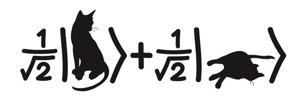
              julia> ( Z₁⊗X₂+Y₁⊗Y₁ ) / √2
              0.707 (|Y₁⟩|Y₁⟩+|Z₁⟩|X₂⟩)
Symbolic to Numeric Conversion
              julia> express( ( Z₁⊗X₂+Y₁⊗Y₁ ) / √2 )
              Ket(dim=4)
                basis: [Spin(1/2) ⊗ Spin(1/2)]
                 0.8535533905932736 + 0.0im
                                0.0 + 0.3535533905932737im
               -0.49999999999999994 + 0.3535533905932737im
                -0.3535533905932737 + 0.0im
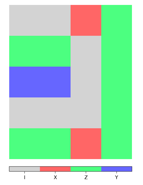
              julia> express( Y₁⊗Y₂, CliffordRepr() )
              Rank 2 stabilizer
              + Z_
              + _Z
              ════
              + Y_
              - _Y
              ════
Play with it at areweentangledyet.com
Other features...
Declarative specification of "imperfections"
Discrete event scheduling
Traveling wavepackets modeling
More formalisms
More symbolic algebra
Digital twin / surrogate modeling
QuantumSavory.jl
github.com/QuantumSavory/QuantumSavory.jl
A few state-of-the-art Simulators
Most sophisticated Clifford algebra simulator
github.com/QuantumSavory/QuantumClifford.jl Multiplying two 1 gigaqubit Paulis in 32 ms.With upcoming "Google Summer of Code" contributors working on GPU acceleration and ECC zoo.
MIT and UMass students working on code generators.
Incoming master student working on code decoders.
Faster-than-Clifford Bell Pair circuits
github.com/QuantumSavory/BPGates.jl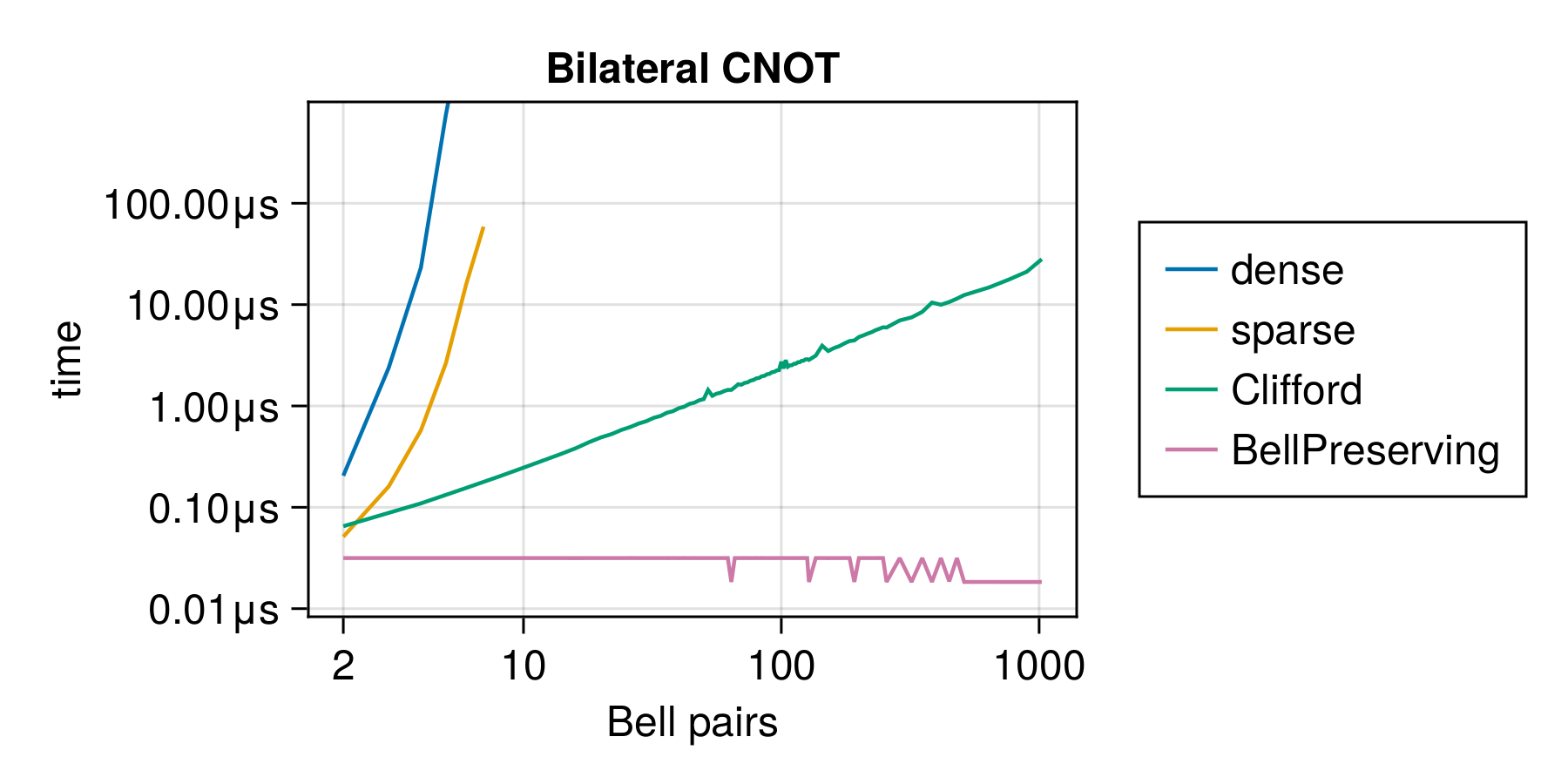
Waveguide Quantum Electrodynamics
github.com/qojulia/WaveguideQED.jl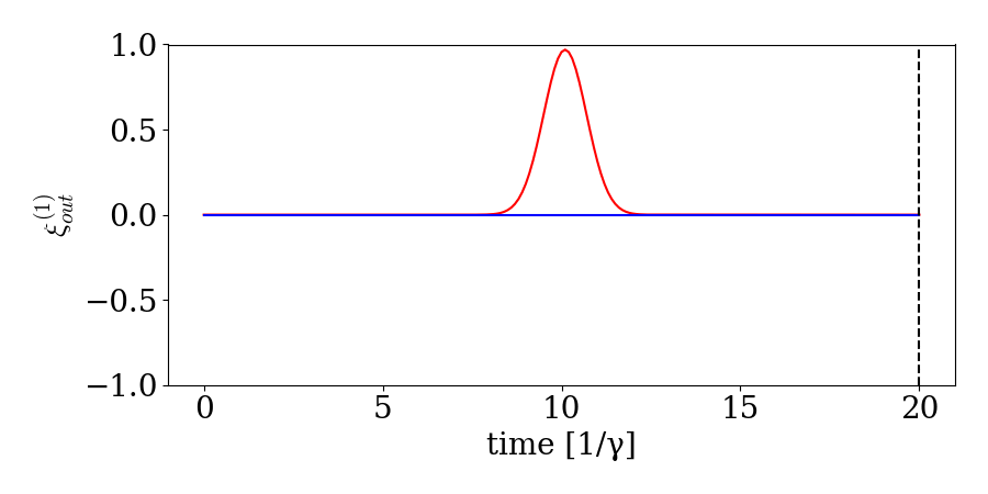
Taking Optimization Seriously
Even your Monte Carlo simulations should be "differentiable"!¹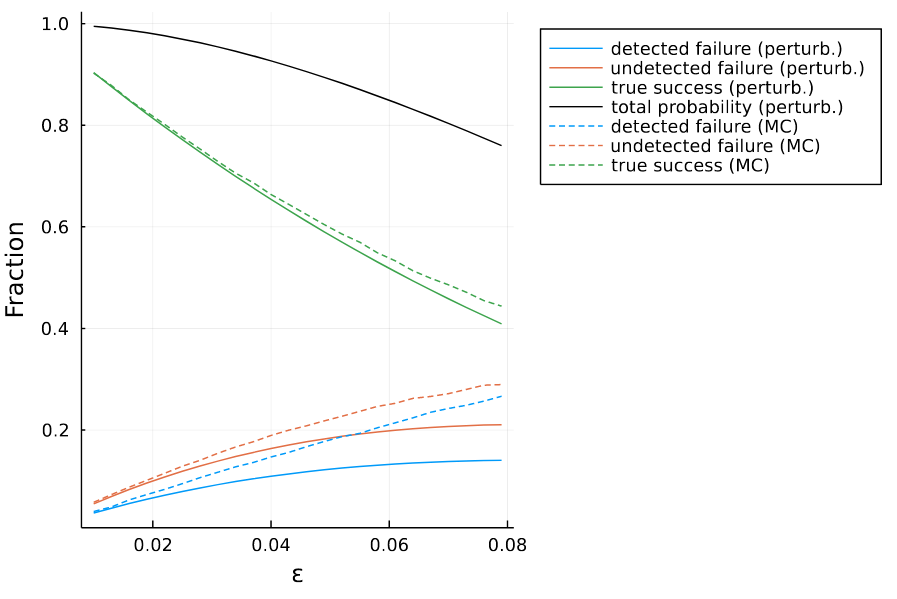
QuantumSavory.jl
github.com/QuantumSavory/QuantumSavory.jl
message me at
stefan@krastanov.org
skrastanov@umass.edu
stefankr@mit.edu
stefan@krastanov.org
skrastanov@umass.edu
stefankr@mit.edu