From Better Entanglement Distillation to Multi-formalism Quantum Simulation Tools for the Entire Network Stack
 Stefan Krastanov
MIT ⟶ UMass Amherst
The Quantum Technology Stack
Materials
Analog Control
Noisy Digital Circuits
Error Correction
Quantum Algorithms
Optimizing Entanglement Distilation
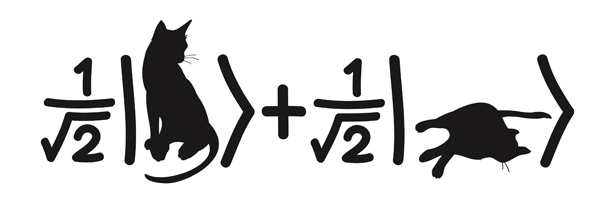
- Krastanov et al.Art installation on Non-contextual Hidden Variable theories
They can be noisy!
Desired:
\[\begin{aligned} A=\frac{|00\rangle+|11\rangle}{\sqrt{2}}\\ \end{aligned}\]The hardware generated:
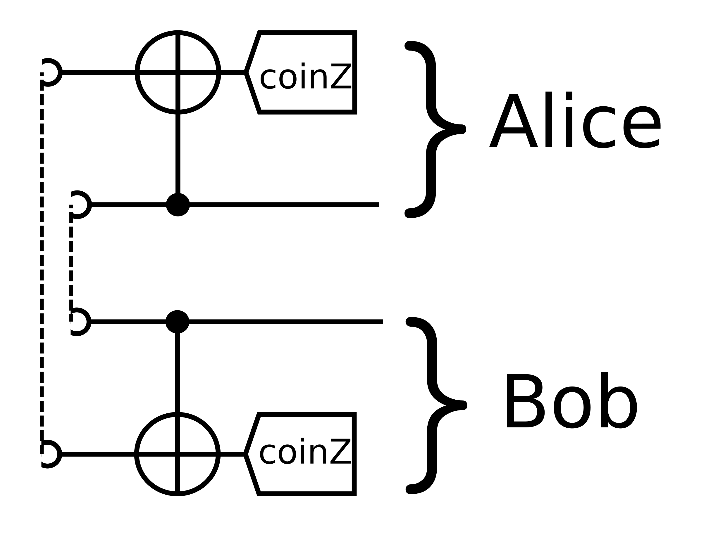
90% chance for \[\begin{aligned} A=\frac{|00\rangle+|11\rangle}{\sqrt{2}}\\ \end{aligned}\] 10% chance for a bit flip on Bob's qubit \[\begin{aligned} C=\frac{|01\rangle+|10\rangle}{\sqrt{2}}\\ \end{aligned}\]Purification of entanglement
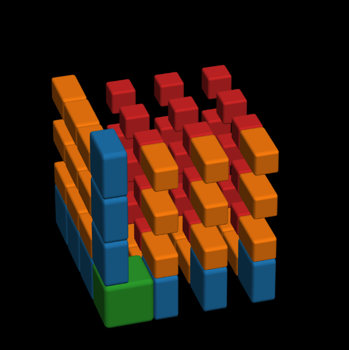
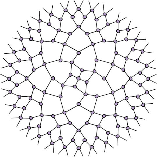
A convenient representation for the density matrix
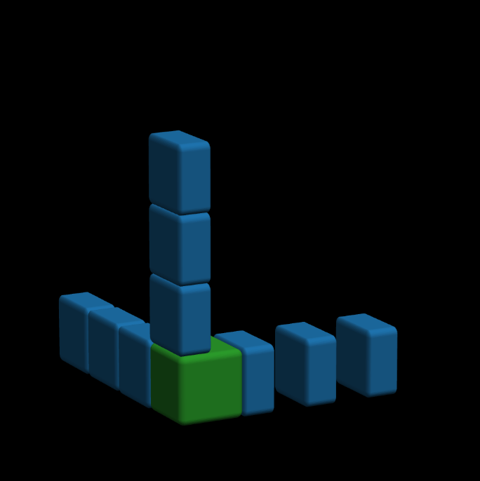
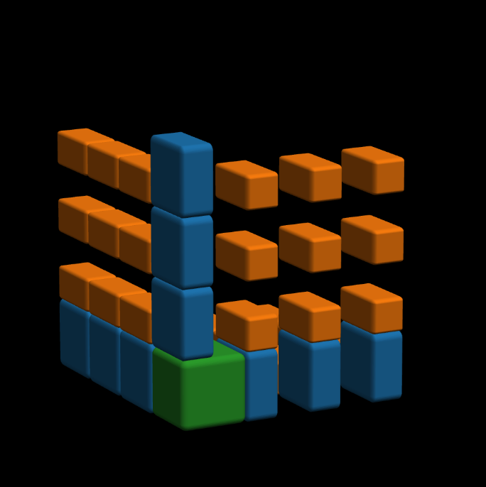
A hypercube of probabilities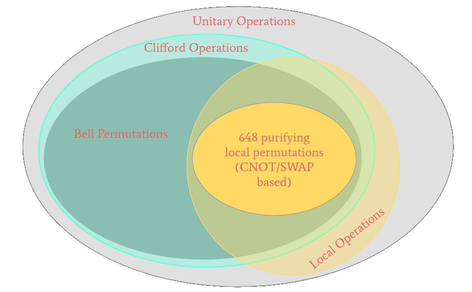
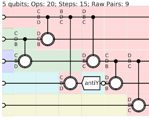
What if we want multi-sacrifice circuit?
Discrete Optimization: Evolutionary Algorithm
Discrete Optimization: Evolutionary Algorithm
Discrete Optimization: Evolutionary Algorithm
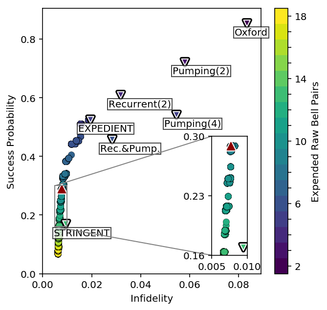
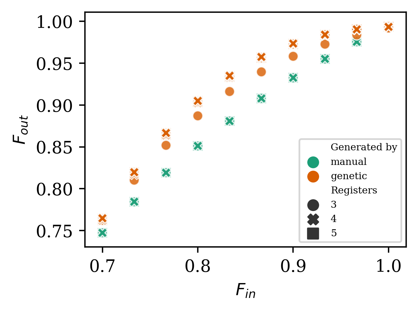
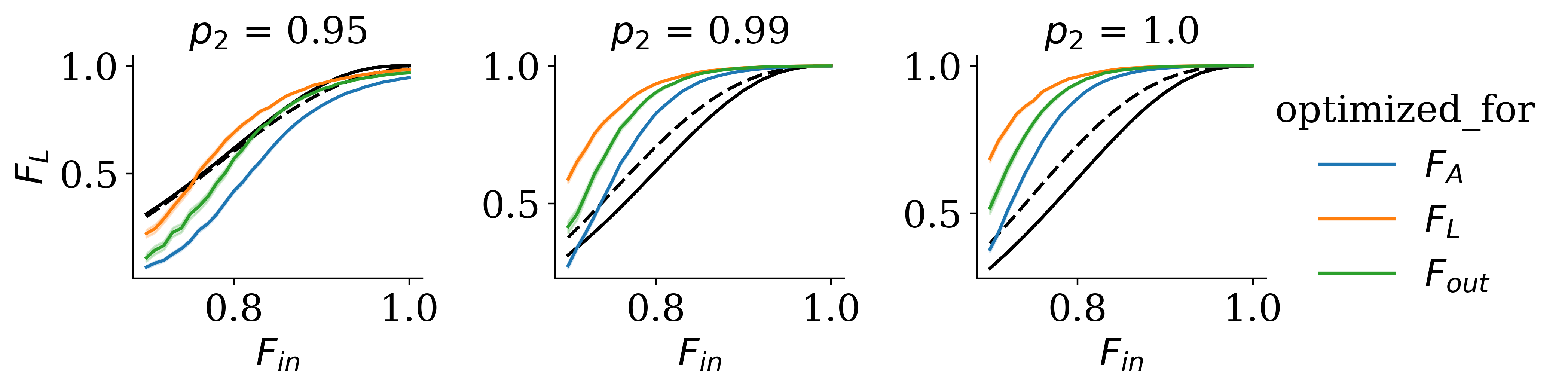
- Krastanov et al.Optimized Entanglement Purification
- Jansen et al.Enumerating all bilocal Clifford distillation protocols through symmetry reduction
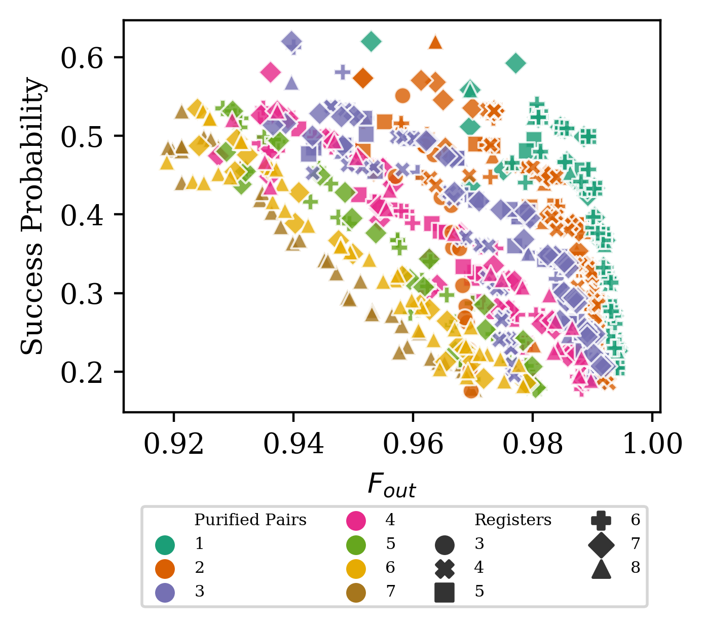
n-to-k purification protocols¹
- Vaishnavi Addala, Stefan Krastanov
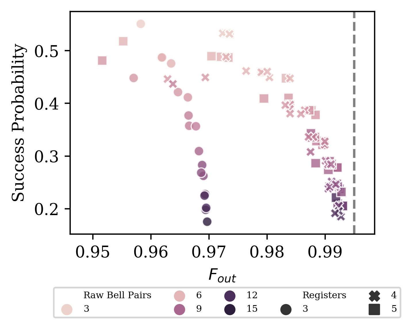
Optimizatin of concatenated
purification ⟶ ECC teleportation
protocols¹
- Vaishnavi Addala, Stefan Krastanov
Modeling Entanglement More Efficiently¹
- Shu Ge, Stefan Krastanov
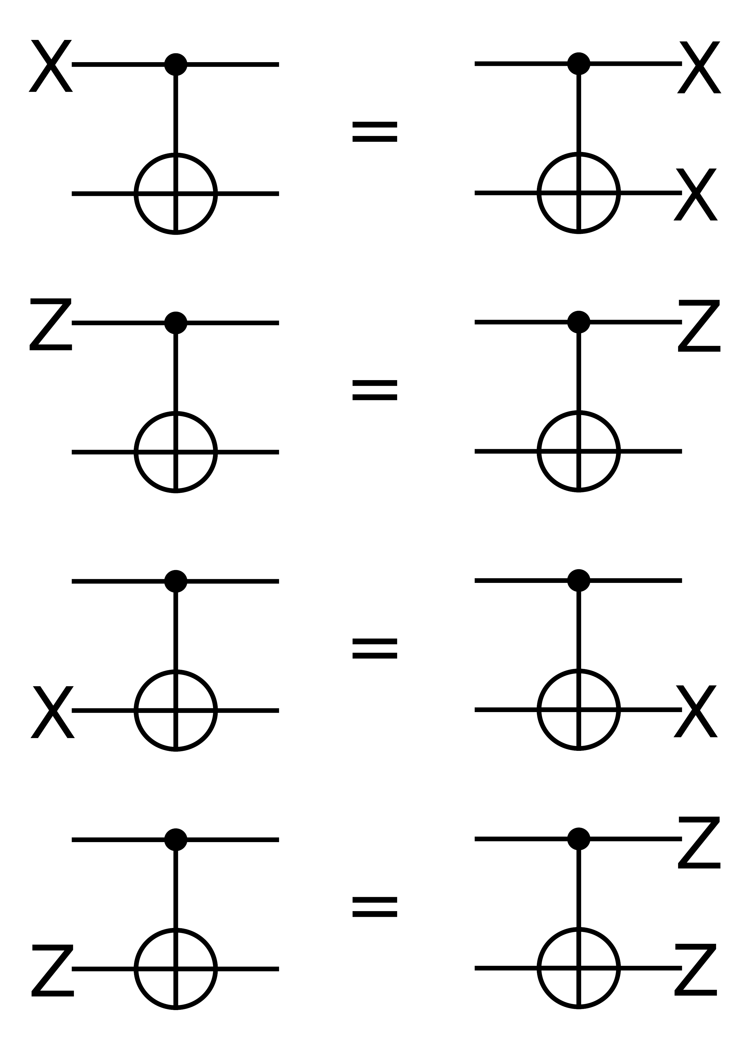
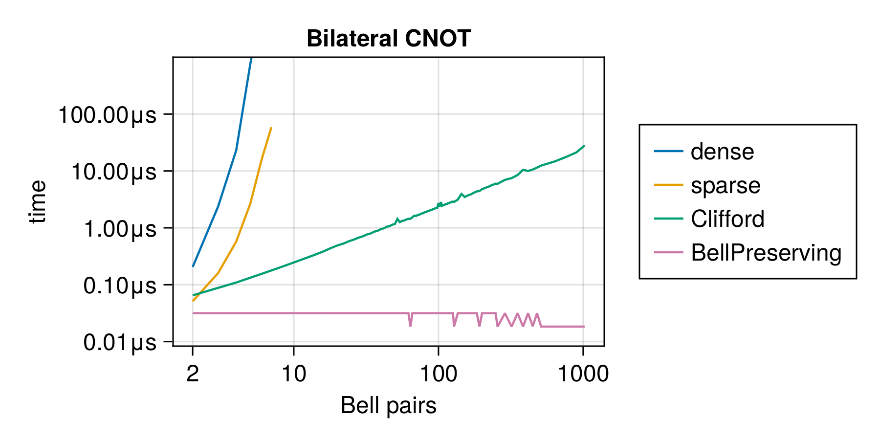
Error-detection circuits are Clifford circuits
Clifford circuits are efficient to simulate on stabilizer states\[ \underbrace{A\otimes B\dots}_{n\text{ pairs}} \]
\[ \left.\begin{pmatrix}0\\1\\0\\\vdots\\0\end{pmatrix}\right\}\scriptsize \mathcal{O}(2^n) \]
\[ \left.\begin{bmatrix}+&XX&\\+&ZZ&\\&&\ddots\end{bmatrix}\right\}\scriptsize \mathcal{O}(n\times n) \]
\[ \underbrace{0011\dots}_{2n \text{ bits}} \]
- Let us call them "Bell Permuting" or "Bell Preserving" gates
- Let us denote them $\mathrm{BP}(n)$
- Permuting gates are Clifford gates
- Not all permutations are local
- Are there Non-Clifford gates that are useful for distillation?
i.e. any $\mathcal{C}_n$ gate can be written as
$C.P\ |\ P\in\mathcal{P}_n\,,C\in\mathcal{C}^*_n$
which provides 20 "distinct" two-qubit gates
- Jansen et al.Enumerating all bilocal Clifford distillation protocols through symmetry reduction
- Dehaene et al.Local permutations of products of Bell states and entanglement distillation
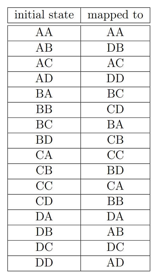
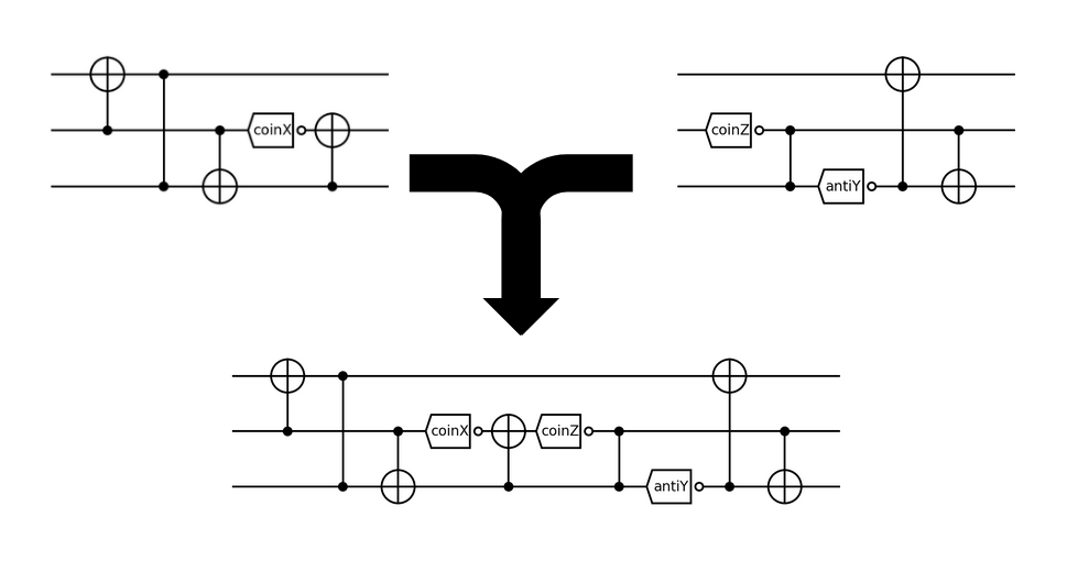
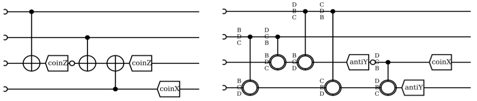
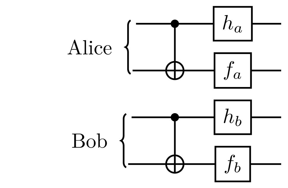
Bell Preserving (bi-local) gates on 2 Bell pairs
where $p\in\mathcal{P}_2$
$h\in\mathcal{C}^*_1$ and $f\in\mathcal{C}^*_1$ and $g_0\in Q$
Bell Preserving (bi-local) gates on 2 Bell pairs
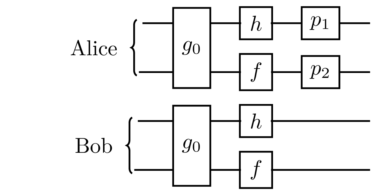
(4 possibilities each)
(6 possibilities each)
Bell Preserving (bi-local) gates
That also maps AA ⟶ AAThere 720 such gates
But just 36 suffice for state of the art purification...
Namely the 6 permutations of BCD.
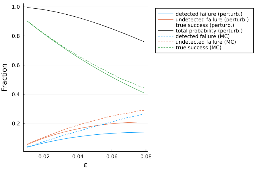
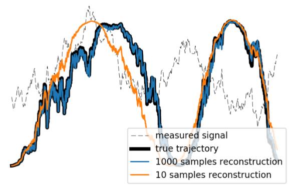
Taking Optimization Seriously
Even your Monte Carlo simulations should be "differentiable"!¹- Arya et al.Automatic Differentiation of Programs with Discrete Randomness
Full-Stack Design and Optimization Toolkit
Types of Dynamics
Types of Dynamics
Hamiltonians, Master Equations
Types of Dynamics
Hamiltonians, Master Equations
Gates, Circuits
Types of Dynamics
Hamiltonians, Master Equations
Gates, Circuits
Weak Measurements, Feedback
State Representation
                traits = [Qubit(), Qubit(), Qumode()]
                reg = Register(traits)

A register "stores" the states being simulated.
                graph = grid([2,3])
                registers = [...]
                net = RegisterNet(graph, registers)
A "graph" of registers can represent a network.
initialize!(reg[1], X₁)
A register's slot can be initialized to an arbitrary state, e.g. $|x_1\rangle$ an eigenstate of $\hat{\sigma}_x$.
                initialize!(reg[1], X₁)
                initialize!(reg[2], Z₁)
                apply!((reg[1], reg[2]), CNOT)
Arbitrary quantum gates or channels can be applied.
              project_traceout!(reg[1], σˣ) # Projective measurement

              observable((reg[1],reg[2]), σᶻ⊗σˣ) # Calculate an expectation
Measurements and expectation values...
Full Symbolic Computer Algebra System
              julia> Z₁
              |Z₁⟩
              julia> ( Z₁⊗X₂+Y₁⊗Y₁ ) / √2
              0.707 (|Y₁⟩|Y₁⟩+|Z₁⟩|X₂⟩)
Symbolic to Numeric Conversion
              julia> express( ( Z₁⊗X₂+Y₁⊗Y₁ ) / √2 )
              Ket(dim=4)
                basis: [Spin(1/2) ⊗ Spin(1/2)]
                 0.8535533905932736 + 0.0im
                                0.0 + 0.3535533905932737im
               -0.49999999999999994 + 0.3535533905932737im
                -0.3535533905932737 + 0.0im
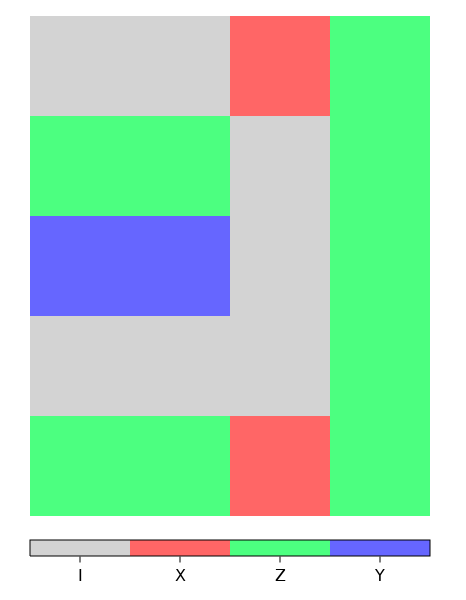
              julia> express( Y₁⊗Y₂, CliffordRepr() )
              Rank 2 stabilizer
              + Z_
              + _Z
              ════
              + Y_
              - _Y
              ════
              for (;src, dst) in edges(mgraph)
                  @process entangler(sim, mgraph, src, dst, ...)
              end
              for node in vertices(mgraph)
                  @process swapper(sim, mgraph, node, ...)
              end
              for (;src, dst) in all_node_pairs(mgraph)
                  @process entangler(sim, mgraph, src, dst, ...)
              end
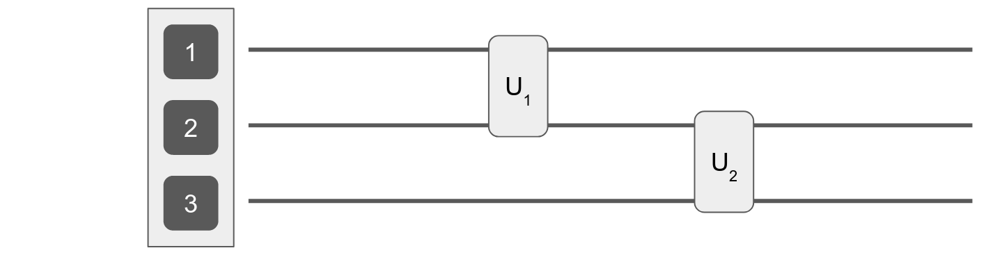
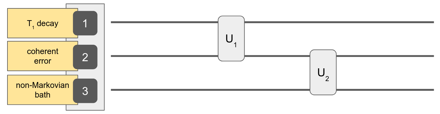
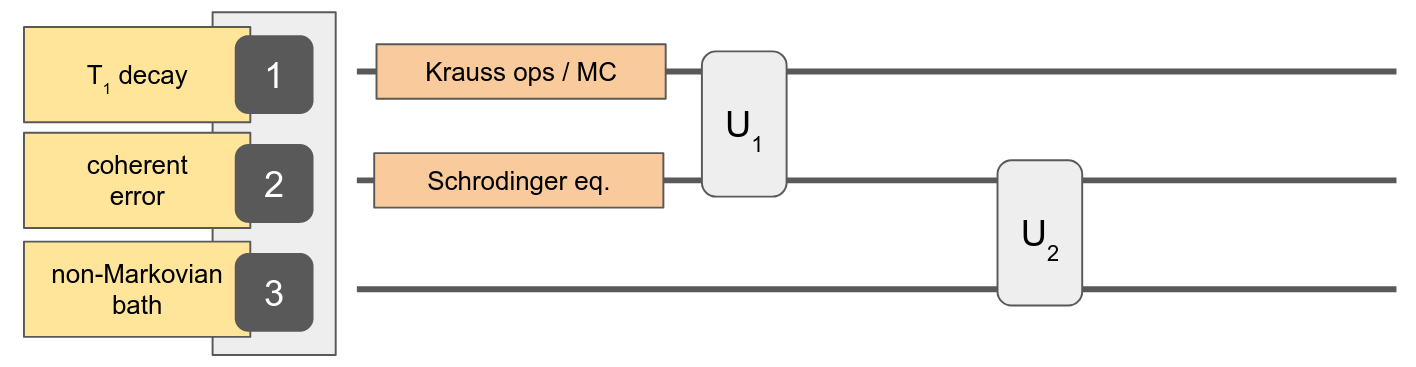
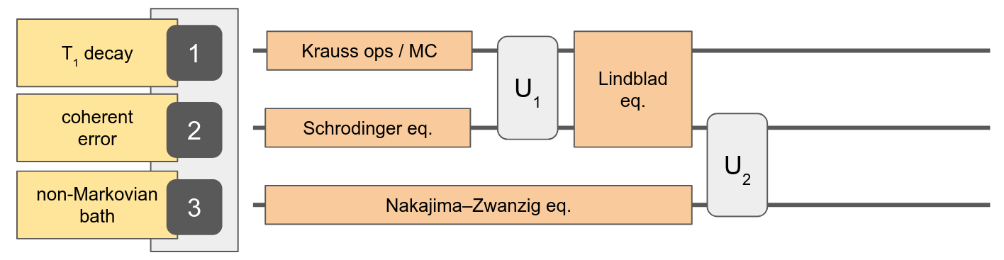
Automatic tracking of noise processes
reg = Register([Qubit(), Qubit(), Qubit()])
                reg = Register(
                  [Qubit(), Qubit(), Qubit()]
                  [T1Decay(T₁), CoherentError(ε*σᶻ), NZ(...)]
                )
                reg = Register(
                  [Qubit(), Qubit(), Qubit()]
                  [T1Decay(T₁), CoherentError(ε*σᶻ), NZ(...)]
                )
                apply!((reg[1],reg[2]), CNOT; time=τ₁)
                reg = Register(
                  [Qubit(), Qubit(), Qubit()]
                  [T1Decay(T₁), CoherentError(ε*σᶻ), NZ(...)]
                )
                apply!((reg[1],reg[2]), CNOT; time=τ₁)
                apply!((reg[2],reg[3]), CPHASE; time=τ₂)
Other features...
Declarative specification of "imperfections"
Discrete event scheduling
Traveling wavepackets modeling
More formalisms
More symbolic algebra
Digital twin / surrogate modeling
QuantumSavory.jl
github.com/Krastanov/QuantumSavory.jl
Better modeling and better optimization for entanglement exist
Try out QuantumClifford.jl - it is public and stable
Be an early tester for QuantumSavory.jl
Including work done by Vaishnavi Addala and Shu Ge, in coordination with Dirk Englund.
Consider gradschool or postdoc at UMass Amherst:

Design of optical/mechanical/spin devices with Sandia, Mitre, and MIT.
Working on practical LDPC ECC in networking and computing.
Creating new tools for the entire community.